Image Classification using Convolutional Neural Networks - Pytorch


Exploring the CIFAR10 Dataset
CIFAR-10 is an established computer-vision dataset used for object recognition. It is a subset of the 80 million tiny images dataset and consists of 60,000 32x32 color images containing one of 10 object classes, with 6000 images per class. It was collected by Alex Krizhevsky, Vinod Nair, and Geoffrey Hinton.
Link:- https://www.kaggle.com/c/cifar-10
Dataset-credentials:- https://www.cs.toronto.edu/~kriz/cifar.html

Importing Libraries
import os
import torch
import torchvision
import tarfile
from torchvision.datasets.utils import download_url
from torch.utils.data import random_split
project_name = 'cifar10-cnn'
dataset_url = "https://s3.amazonaws.com/fast-ai-imageclas/cifar10.tgz"
download_url(dataset_url, '.')
with tarfile.open('./cifar10.tgz', 'r:gz') as tar:              # r:gz --> read mode in g zip format
    tar.extractall(path='./data')
data_dir = './data/cifar10'

print(os.listdir(data_dir))
classes = os.listdir(data_dir + "/train")
print(classes)
airplane_files = os.listdir(data_dir + "/train/airplane")
print("No. of test examples for airplanes: ", len(airplane_files))
print(airplane_files[:5])
ship_test_files = os.listdir(data_dir + "/test/ship")
print("No of test examples for ship:", len(ship_test_files))
print(ship_test_files[10:50])
from torchvision.datasets import ImageFolder
from torchvision.transforms import ToTensor
dataset = ImageFolder(data_dir + '/train', transform = ToTensor())
img, label = dataset[0]
print(img.shape, label)
img[2]                            # img tensor
print(dataset.classes)
import matplotlib
import matplotlib.pyplot as plt
%matplotlib inline

matplotlib.rcParams['figure.facecolor'] = '#ffffff'
def show_example(img, label):
    print('Label: ', dataset.classes[label], "("+str(label)+")")
    plt.imshow(img.permute(1, 2, 0))                                 # matplot lib expects channels in final dimension
img, label = dataset[5]
show_example(img, label)

show_example(*dataset[0])

show_example(*dataset[1099])

random_seed = 42
torch.manual_seed(random_seed);  # It helps to standardise validation set
val_size = 5000
train_size = len(dataset) - val_size

train_ds, val_ds = random_split(dataset, [train_size, val_size])
len(train_ds), len(val_ds)
from torch.utils.data.dataloader import DataLoader

batch_size = 128
train_dl = DataLoader(train_ds, batch_size, shuffle=True, num_workers=4, pin_memory = True)
val_dl = DataLoader(val_ds, batch_size*2, num_workers = 4, pin_memory = True)
from torchvision.utils import make_grid

def show_batch(dl):
    for images, labels in dl:
        fig, ax = plt.subplots(figsize = (12, 6))
        ax.set_xticks([]); ax.set_yticks([])
        ax.imshow(make_grid(images, nrow=16).permute(1, 2, 0))
        break
show_batch(train_dl)

nn.Linear gives full connected layer architecture nn.Conv2d gives convolutional neural network
Basic working of CNN can be described as follows :

Working of kernel can be describes as :
Implementation of a convolution operation on a 1 channel image with a 3x3 kernel
def apply_kernel(image, kernel):
    ri, ci = image.shape           #image dimension
    rk, ck = kernel.shape          #kernel dimension
    ro, co = ri-rk+1, ci-ck+1      #output dimension
    output = torch.zeros([ro, co])

    for i in range(ro):
        for j in range(co):
            output[i, j] = torch.sum(image[i:i+rk, j:j+ck] * kernel)
    return output
sample_image = torch.tensor([
    [0, 0, 75, 80, 80],
    [0, 75, 80, 80, 80],
    [0, 75, 80, 80, 80],
    [0, 70, 75, 80, 80],
    [0, 0, 0, 0, 0]
], dtype = torch.float32)


sample_kernel = torch.tensor([
    [-1, -2, -1],
    [0, 0, 0],
    [1, 2, 1]
], dtype = torch.float32)

apply_kernel(sample_image, sample_kernel)
Refer this blog post for more in-depth intution of CNN :- Convolution in depth
Observation : 5x5 image got reduced to a 3x3 output, while kernel in running over internal values multiple times, but still values of corner are covered only once, so we'll use padding and it will return output as the same size as input
Padding can be understood using following diagram:
Now we have moved kernel by 1 position each time, we can move kernel by 2 positons too, this is call Stride
Stride can be understood using folloeing diagram:

For multi-channel images, a different kernel is applied to each channels, and the outputs are added together pixel-wise.
There are certain advantages offered by convolutional layers when working with image data:
- Fewer parameters: A small set of parameters (the kernel) is used to calculate outputs of the entire image, so the model has much fewer parameters compared to a fully connected layer.
- Sparsity of connections: In each layer, each output element only depends on a small number of input elements, which makes the forward and backward passes more efficient.
- Parameter sharing and spatial invariance: The features learned by a kernel in one part of the image can be used to detect similar pattern in a different part of another image.
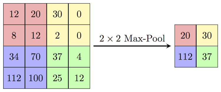
We will also use a max-pooling layers to progressively decrease the height & width of the output tensors from each convolutional layer.
import torch.nn as nn
import torch.nn.functional as F
conv = nn.Conv2d(3, 8, kernel_size = 3, stride = 1, padding = 1) # 8 is no of kernels which also descide no of output channels ie feature map
pool = nn.MaxPool2d(2, 2)
for images, labels in train_dl:
    print('images.shape:', images.shape)
    out = conv(images)

    print('output.shape:', out.shape)

    out = pool(out)

    print('max-pool output.shape:', out.shape)       # max pool will reduce size

    break
conv.weight.shape # we have 8 kernel and each kernel contain 3 matrices for 3 input channel and each of 3 matrix have 3x3 matrix that is gonna slide
conv.weight[0, 0]
conv.weight[0]
simple_model = nn.Sequential(
    nn.Conv2d(3, 8, kernel_size=3, stride=1, padding=1),
    nn.MaxPool2d(2,2)
)
for images, labels, in train_dl:
    print('images.shape:', images.shape)
    out = simple_model(images)
    print('out.shape:', out.shape)
    break

class ImageClassificationBase(nn.Module):

    def training_step(self, batch):
        images, labels = batch
        out = self(images)
        loss = F.cross_entropy(out, labels)
        return loss

    def validation_step(self, batch):
        images, labels = batch
        out = self(images)
        loss = F.cross_entropy(out, labels)
        acc = accuracy(out, labels)
        return {'val_loss': loss.detach(), 'val_acc': acc}

    def validation_epoch_end(self, outputs):
        batch_losses = [x['val_loss'] for x in outputs]
        epoch_loss = torch.stack(batch_losses).mean()
        batch_accs = [x['val_acc'] for x in outputs]
        epoch_acc = torch.stack(batch_accs).mean()
        return {'val_loss': epoch_loss.item(), 'val_acc': epoch_acc.item()}

    def epoch_end(self, epoch, result):
        print("Epoch [{}], train_loss: {:.4f}, val_loss: {:.4f}, val_acc: {:.4f}".format(epoch, result['train_loss'], result['val_loss'], result['val_acc']))

def accuracy(outputs, labels):
    _, preds = torch.max(outputs, dim=1)
    return torch.tensor(torch.sum(preds == labels).item() / len(preds))
class Cifar10CnnModel(ImageClassificationBase):

    def __init__(self):
        super().__init__()
        self.network = nn.Sequential(
        # input: 3 x 32 x 32
        nn.Conv2d(3, 32, kernel_size=3, padding=1),  # i/p 3 channels, applies 32 kernels to create o/p: 32 x 32
        # output: 32 x 32 x 32
        nn.ReLU(),
        nn.Conv2d(32, 64, kernel_size=3, stride=1, padding=1),
        # output: 64 x 32 x 32
        nn.ReLU(),
        nn.MaxPool2d(2, 2), # 32 x 32 --> 16 x 16

        #output 64 x 16 x 16

        nn.Conv2d(64, 128, kernel_size=3, stride=1, padding=1),
        nn.ReLU(),
        nn.Conv2d(128, 128, kernel_size=3, stride=1, padding=1),
        nn.ReLU(),
        nn.MaxPool2d(2, 2),  # output 128 x 8 x 8

        nn.Conv2d(128, 256, kernel_size=3, stride=1, padding=1),
        nn.ReLU(),
        nn.Conv2d(256, 256, kernel_size=3, stride=1, padding=1),
        nn.ReLU(),
        nn.MaxPool2d(2, 2),  # output 256 x 4 x 4

        nn.Flatten(),              # take 256x4x4 o/p feature map and flatten it out into a vector
        nn.Linear(256*4*4, 1024),
        nn.ReLU(),
        nn.Linear(1024, 512),
        nn.ReLU(),
        nn.Linear(512, 10))

    def forward(self, xb):
        return self.network(xb)
model = Cifar10CnnModel()
model
Look at out model :

for images, labels in train_dl:
    print('images.shape:', images.shape)
    out = model(images)
    print('out.shape:', out.shape)
    print('out[0]', out[0])               # out will have prob of each classes
    break
def get_default_device():

    if torch.cuda.is_available():
        return torch.device('cuda')
    else:
        return torch.device('cpu')
device = get_default_device()
device
def to_device(data, device):
    """Move tensors to chosen device"""
    if isinstance(data, (list,tuple)):
        return [to_device(x, device) for x in data]
    return data.to(device, non_blocking = True)       # to method
class DeviceDataLoader():

    def __init__(self, dl, device):
        self.dl = dl
        self.device = device

    def __iter__(self):
        for b in self.dl:
            yield to_device(b, self.device)

    def __len__(self):
        return len(self.dl)
train_dl = DeviceDataLoader(train_dl, device)
val_dl = DeviceDataLoader(val_dl, device)
to_device(model, device);
@torch.no_grad() # tells when evaluate is being executed we dont want to compute any gradient
def evaluate(model, val_loader):
    model.eval()    # tells pytorch that these layers should be put into validation mode
    outputs = [model.validation_step(batch) for batch in val_loader]
    return model.validation_epoch_end(outputs)

def fit(epochs, lr, model, train_loader, val_loader, opt_func = torch.optim.SGD):
    history = []
    optimizer = opt_func(model.parameters(), lr)
    for epoch in range(epochs):
        # Training Phase
        model.train()      # tells pytorch that these layers should be put into training mode
        train_losses = []
        for batch in train_loader:
            loss = model.training_step(batch)
            train_losses.append(loss)
            loss.backward()
            optimizer.step()
            optimizer.zero_grad()
        # Validation Phase
        result = evaluate(model, val_loader)
        result['train_loss'] = torch.stack(train_losses).mean().item()
        model.epoch_end(epoch, result)
        history.append(result)
    return history
model = to_device(Cifar10CnnModel(), device)
evaluate(model, val_dl) # with initial set of parameters --> random result
num_epochs = 10
opt_func = torch.optim.Adam
lr = 0.001
history = fit(num_epochs, lr, model, train_dl, val_dl, opt_func)
def plot_accuracies(history):
    accuracies = [x['val_acc'] for x in history]
    plt.plot(accuracies, '-x')
    plt.xlabel('epoch')
    plt.ylabel('accuracy')
    plt.title('Accuracy vs. No. of epochs');
plot_accuracies(history)

def plot_losses(history):
    train_losses = [x.get('train_loss') for x in history]
    val_losses = [x['val_loss'] for x in history]
    plt.plot(train_losses, '-x')
    plt.plot(val_losses, '-rx')
    plt.xlabel('epoch')
    plt.ylabel('loss')
    plt.legend(['Training', 'Validation'])
    plt.title('Loss vs No of epochs')
plot_losses(history)

Training error goes down and val error getting up after some time : overfitting
example:
test_dataset = ImageFolder(data_dir+'/test', transform=ToTensor())
def predict_image(img, model):
    xb = to_device(img.unsqueeze(0), device)      # convert to batch of 1
    yb = model(xb)                                # get predictions from model
    _, preds = torch.max(yb, dim=1)               # pick max probab
    return dataset.classes[preds[0].item()]       # retrive label
img, label = test_dataset[1]
plt.imshow(img.permute(1, 2, 0))
print('Label:', dataset.classes[label], ', Predicted:', predict_image(img, model))

img, label = test_dataset[1002]
plt.imshow(img.permute(1, 2, 0))
print('Label:', dataset.classes[label], ', Predicted:', predict_image(img, model))

img, label = test_dataset[0]
plt.imshow(img.permute(1, 2, 0))
print('Label:', dataset.classes[label], ', Predicted:', predict_image(img, model))

img, label = test_dataset[6153]
plt.imshow(img.permute(1, 2, 0))
print('Label:', dataset.classes[label], ', Predicted:', predict_image(img, model))

test_loader = DeviceDataLoader(DataLoader(test_dataset, batch_size*2), device)
result = evaluate(model, test_loader)
result
torch.save(model.state_dict(), 'cifar10-cnn.pth')