Classifying Cifar-10 using ResNets - Pytorch


Understanding use of Regularization and Data Augmentation
Exploring the CIFAR10 Dataset
CIFAR-10 is an established computer-vision dataset used for object recognition. It is a subset of the 80 million tiny images dataset and consists of 60,000 32x32 color images containing one of 10 object classes, with 6000 images per class. It was collected by Alex Krizhevsky, Vinod Nair, and Geoffrey Hinton.
Link:- https://www.kaggle.com/c/cifar-10
Dataset-credentials:- https://www.cs.toronto.edu/~kriz/cifar.html

import os
import torch
import torchvision
import tarfile
import torch.nn as nn
import numpy as np
import torch.nn.functional as F
from torchvision.datasets.utils import download_url
from torchvision.datasets import ImageFolder
from torch.utils.data import DataLoader
import torchvision.transforms as tt
from torch.utils.data import random_split
from torchvision.utils import make_grid
import matplotlib
import matplotlib.pyplot as plt
%matplotlib inline

matplotlib.rcParams['figure.facecolor'] = '#ffffff'
project_name = 'cifar10-resnet'
data_dir = './data/cifar10'
print(os.listdir(data_dir))
classes = os.listdir(data_dir + "/train")
print(classes)
Data Preprocessing
going to use test set for validation
Channel wise data normalisation
we will normalize the image tensors by substracting the mean and dividing by the standard deviation across each channel. it will mean the data across each channel to 0 and standard deviation to 1. normalizing data prevents the values from any one channel from disproportionately affecting the losses and gradients while training simply by having a higher or wider range of values that others

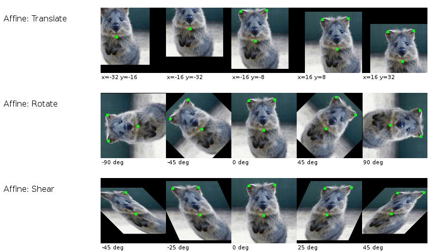
Randomized data augmentation
Applying chosen transformations while loading images from the training dataset. we will pad each image by 4 pixels and then take a random crop of size 32 x 32 and then flip the image horizontly with a 50% probability. Since the transformation will be applied randomly and dynamically each time a particular image is loaded, the model sees slightly different images in each epoch of training, which allows it generalize better
stats = ((0.4914, 0.4822, 0.4465), (0.2023, 0.1994, 0.2010))

train_tfms = tt.Compose([tt.RandomCrop(32, padding=4, padding_mode='reflect'), # it is going to shift the image around upto 4 pixels(top/bottom/left/right) each time
                         tt.RandomHorizontalFlip(), # default probab = 0.5
                         #tt.RandomRotation(),
                         #tt.RandomResizedCrop(256, scale=(0.5, 0.9), ratio=(1, 1)),
                         #tt.ColorJitter(brightness=0.1, contrast =0.1, saturation=0.1),
                         tt.ToTensor(),
                         tt.Normalize(*stats, inplace=True)])

valid_tfms = tt.Compose([tt.ToTensor(), tt.Normalize(*stats)])

# we can not apply transformations to validation set coz it is for testing on real data
we need normalized transformation for validation set too bcoz when we train the model using normalized data then model no longer understands the original pixel values, it only understands the mormalize pixel values which has been shifted using mean and standard deviations, therefore any new input that is used should also contain same normalization
train_ds = ImageFolder(data_dir+'/train', train_tfms)
valid_ds = ImageFolder(data_dir+'/test', valid_tfms)
batch_size = 400
train_dl = DataLoader(train_ds, batch_size, shuffle=True, num_workers=3, pin_memory=True)
valid_dl = DataLoader(valid_ds, batch_size*2, num_workers=3, pin_memory=True)
def denormalize(images, means, stds):
    means = torch.tensor(means).reshape(1, 3, 1, 1)
    stds = torch.tensor(stds).reshape(1, 3, 1, 1)
    return images * stds + means

def show_batch(dl):
    for images, labels in dl:
        fig, ax = plt.subplots(figsize=(12, 12))
        ax.set_xticks([]); ax.set_yticks([])
        denorm_images = denormalize(images, *stats)
        ax.imshow(make_grid(denorm_images[:64], nrow=8).permute(1, 2, 0).clamp(0, 1))
        break
show_batch(train_dl)

def get_default_device():

    if torch.cuda.is_available():
        return torch.device('cuda')
    else:
        return torch.device('cpu')
device = get_default_device()
device
def to_device(data, device):
    """Move tensors to chosen device"""
    if isinstance(data, (list,tuple)):
        return [to_device(x, device) for x in data]
    return data.to(device, non_blocking = True)       # to method
class DeviceDataLoader():

    def __init__(self, dl, device):
        self.dl = dl
        self.device = device

    def __iter__(self):
        for b in self.dl:
            yield to_device(b, self.device)

    def __len__(self):
        return len(self.dl)
train_dl = DeviceDataLoader(train_dl, device)
valid_dl = DeviceDataLoader(valid_dl, device)
we will add residual block, that adds the original input back to the output feature map obtained by passing the input through one or more conv layers
without residual block, these layers are responsible for transforming the input into the output, our entire network in responsible for transforming images 3d rgb 32x32 color images into 10 output class probabilities but when we pass a residual layer then our conv layers are no longer responsible for converting the i/p to o/p rather they only have to calculate the difference between i/p and o/p coz, final o/p is the o/p of covn layer + i/p so simply o/p of conv layer is desired op - i/p layer
so the wieghts can learn more powerful features

class SimpleResidualBlock(nn.Module):
    def __init__(self):
        super().__init__()
        self.conv1 = nn.Conv2d(in_channels=3, out_channels=3, kernel_size=3, stride=1, padding=1)
        self.relu1 = nn.ReLU()
        self.conv2 = nn.Conv2d(in_channels=3, out_channels=3, kernel_size=3, stride=1, padding=1)
        self.relu2 = nn.ReLU()
# in a residual block we can not change the no of o/p channels, coz if we change it ex to 128 then we'll not be able to add the orginal i/p to o/p coz then i/p shape and o/p shape would not match
    def forward(self, x):
        out = self.conv1(x)
        out = self.relu1(out)
        out = self.conv2(out)
        return self.relu2(out) + x
simple_resnet = to_device(SimpleResidualBlock(), device)

for images, labels in train_dl:
    print(images.shape)
    out = simple_resnet(images)
    print(out.shape)
    break

del simple_resnet, images, labels
torch.cuda.empty_cache()
Batch Normalization layer: normalizes the o/p of previous layer
some cool resources : Residual blocks Batch Normalization ResNet9
lmao cool animation down there
ResNet34 : 
Cmon dude see some more about ResNets
ResNet18 : 


def accuracy(outputs, labels):
    _, preds = torch.max(outputs, dim=1)
    return torch.tensor(torch.sum(preds == labels).item()/len(preds))

class ImageClassificationBase(nn.Module):
    def training_step(self, batch):
        images, labels = batch
        out = self(images)
        loss = F.cross_entropy(out, labels)
        return loss

    def validation_step(self, batch):
        images, labels = batch
        out = self(images)
        loss = F.cross_entropy(out, labels)
        acc = accuracy(out, labels)
        return {'val_loss': loss.detach(), 'val_acc': acc}

    def validation_epoch_end(self, outputs):
        batch_losses = [x['val_loss'] for x in outputs]
        epoch_loss = torch.stack(batch_losses).mean()
        batch_accs = [x['val_acc'] for x in outputs]
        epoch_acc = torch.stack(batch_accs).mean()
        return {'val_loss': epoch_loss.item(), 'val_acc': epoch_acc.item()}

    def epoch_end(self, epoch, result):
        print("Epoch [{}], last_lr: {:.5f}, train_loss: {:.4f}, val_loss: {:.4f}, val_acc: {:.4f}".format(
               epoch, result['lrs'][-1], result['train_loss'], result['val_loss'], result['val_acc']))
def conv_block(in_channels, out_channels, pool=False):
    layers = [nn.Conv2d(in_channels, out_channels, kernel_size=3, padding=1),
              nn.BatchNorm2d(out_channels),
              nn.ReLU(inplace=True)]

    if pool: layers.append(nn.MaxPool2d(2))
    return nn.Sequential(*layers) # * layers is same as passing one by one args to nn.Sequential

class ResNet9(ImageClassificationBase):
    def __init__(self, in_channels, num_classes):
        super().__init__()
        # 400 x 3 x 32 x 32

        self.conv1 = conv_block(in_channels, 64)                # 64 x 32 x 32
        self.conv2 = conv_block(64, 128, pool=True)            # 128 x 16 x 16
        self.res1 = nn.Sequential(conv_block(128, 128),
                                  conv_block(128, 128))        # 128 x 16 x 16

        self.conv3 = conv_block(128, 256, pool=True)           # 256 x 8 x 8
        self.conv4 = conv_block(256, 512, pool=True)           # 512 x 4 x 4
        self.res2 = nn.Sequential(conv_block(512, 512),
                                  conv_block(512, 512))         # 512 x 4 x 4

        self.classifier = nn.Sequential(nn.MaxPool2d(4),        # 512 x 1 x 1
                                        nn.Flatten(),           # 512
                                        nn.Dropout(0.2),        # 512 -->used to avoid overfitting
                                        nn.Linear(512, num_classes))  # 10

    def forward(self, xb):
        out = self.conv1(xb)
        out = self.conv2(out)
        out = self.res1(out) + out
        out = self.conv3(out)
        out = self.conv4(out)
        out = self.res2(out) + out
        out = self.classifier(out)
        return out
model = to_device(ResNet9(3, 10), device)
model
Training the model
Before we train the model, we're going to make a bunch of small but important improvements to our fit function:
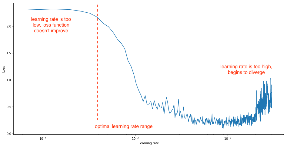
- Learning rate scheduling: Instead of using a fixed learning rate, we will use a learning rate scheduler, which will change the learning rate after every batch of training. There are many strategies for varying the learning rate during training, and the one we'll use is called the "One Cycle Learning Rate Policy", which involves starting with a low learning rate, gradually increasing it batch-by-batch to a high learning rate for about 30% of epochs, then gradually decreasing it to a very low value for the remaining epochs. Learn more: https://sgugger.github.io/the-1cycle-policy.html
Yo start with a low learning rate and then slowly keeps inc lr so that model keeps making larger steps and then start dec the lr again coz once model approaches the good set of weights then we want to narrow down and pick the set of weights by taking really small steps towrds that optimal one

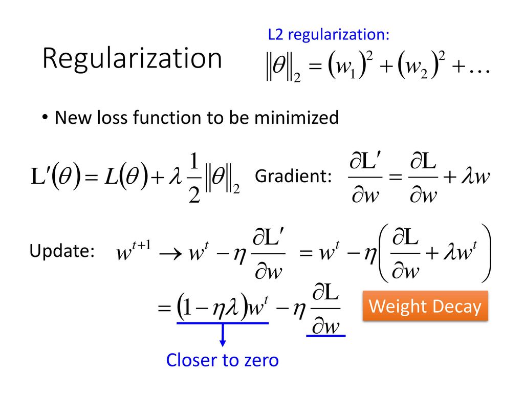
- Weight decay: regularization technique which prevents the weights from becoming too large by adding an additional term to the loss function.Learn more: https://towardsdatascience.com/this-thing-called-weight-decay-a7cd4bcfccab
now Loss = MSE(y_hat, y) + wd * sum(w^2)
When we update weights using gradient descent we do the following:
w(t) = w(t-1) - lr * dLoss / dw
Now since our loss function has 2 terms in it, the derivative of the 2nd term w.r.t w would be:
d(wd w^2) / dw = 2 wd * w (similar to d(x^2)/dx = 2x)
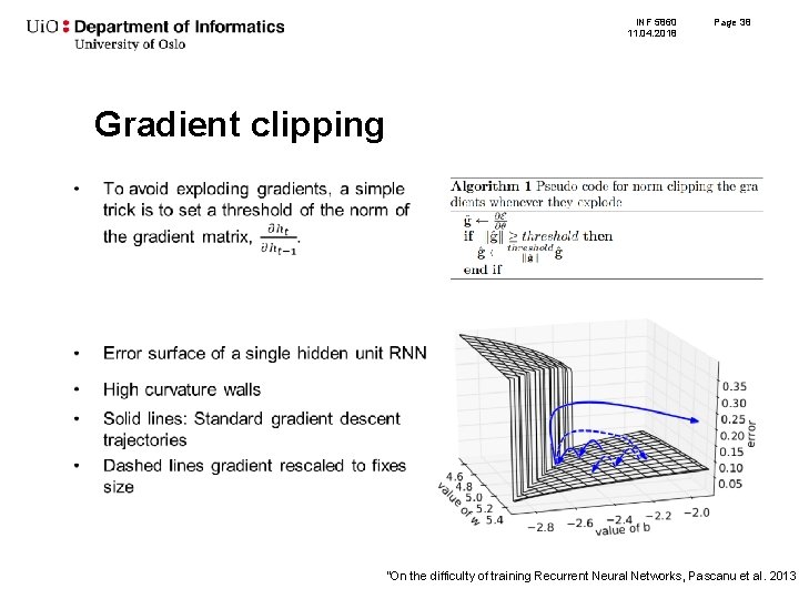
- Gradient clipping: Apart from the layer weights and outputs, it also helpful to limit the values of gradients to a small range to prevent undesirable changes in parameters due to large gradient values. This simple yet effective technique is called gradient clipping. Learn more: https://towardsdatascience.com/what-is-gradient-clipping-b8e815cdfb48

@torch.no_grad()
def evaluate(model, val_loader):
    model.eval()                    # tells model that we are currently evaluating and not training
    outputs = [model.validation_step(batch) for batch in val_loader]
    return model.validation_epoch_end(outputs)

def get_lr(optimizer):
    for param_group in optimizer.param_groups:
        return param_group['lr']

def fit_one_cycle(epochs, max_lr, model, train_loader, val_loader,
                  weight_decay=0, grad_clip=None, opt_func=torch.optim.SGD):
    torch.cuda.empty_cache()
    history =[]

    optimizer = opt_func(model.parameters(), max_lr, weight_decay=weight_decay)

    sched = torch.optim.lr_scheduler.OneCycleLR(optimizer, max_lr, epochs=epochs,
                                                steps_per_epoch=len(train_loader))

    for epoch in range(epochs):
        model.train()
        train_losses= []
        lrs = []
        for batch in train_loader:
            loss = model.training_step(batch)
            train_losses.append(loss)
            loss.backward()

            if grad_clip:
                nn.utils.clip_grad_value_(model.parameters(), grad_clip)

            optimizer.step()
            optimizer.zero_grad()

            lrs.append(get_lr(optimizer))
            sched.step()

        result = evaluate(model, val_loader)
        result['train_loss'] = torch.stack(train_losses).mean().item()
        result['lrs'] = lrs
        model.epoch_end(epoch, result)
        history.append(result)

    return history
history = [evaluate(model, valid_dl)]
history
epochs = 16
max_lr = 0.01
grad_clip = 0.1
weight_decay = 1e-4
opt_func = torch.optim.Adam
%%time

history += fit_one_cycle(epochs, max_lr, model, train_dl, valid_dl,
                         grad_clip=grad_clip, weight_decay = weight_decay)
def plot_accuracies(history):
    accuracies = [x['val_acc'] for x in history]
    plt.plot(accuracies, '-x')
    plt.xlabel('epoch')
    plt.ylabel('accuracy')
    plt.title('Accuracy vs. No. of epochs');
plot_accuracies(history)

def plot_losses(history):
    train_losses = [x.get('train_loss') for x in history]
    val_losses = [x['val_loss'] for x in history]
    plt.plot(train_losses, '-bx')
    plt.plot(val_losses, '-rx')
    plt.xlabel('epoch')
    plt.ylabel('loss')
    plt.legend(['Training', 'Validation'])
    plt.title('Loss vs. No of epochs');
plot_losses(history)

def plot_lrs(history):
    lrs = np.concatenate([x.get('lrs', []) for x in history])
    plt.plot(lrs)
    plt.xlabel('Batch no.')
    plt.ylabel('Learning rate')
    plt.title('Learning Rate vs Batch no.');
plot_lrs(history)

def predict_image(img, model):
    xb = to_device(img.unsqueeze(0), device)
    yb = model(xb)

    _, pred = torch.max(yb, dim=1)

    return train_ds.classes[pred[0].item()]
img, label = valid_ds[2341]
plt.imshow(img.permute(1, 2, 0).clamp(0, 1))
print('Label:', train_ds.classes[label], ', Predicted:', predict_image(img, model))

img, label = valid_ds[1002]
plt.imshow(img.permute(1, 2, 0))
print('Label:', valid_ds.classes[label], ', Predicted:', predict_image(img, model))

img, label = valid_ds[1111]
plt.imshow(img.permute(1, 2, 0))
print('Label:', valid_ds.classes[label], ', Predicted:', predict_image(img, model))

img, label = valid_ds[1921]
plt.imshow(img.permute(1, 2, 0))
print('Label:', valid_ds.classes[label], ', Predicted:', predict_image(img, model))

torch.save(model.state_dict(), 'cifar-10-resnet9.pth')