Time Series Anomaly Detection and LSTM Autoencoder for ECG Data using Pytorch


- Importing Libraries
- Dataset Description
- Exploratory Data Analysis
- LSTM Autoencoder
- LSTM Autoencoder
- Training
- Choosing a threshold
- Evaluation
import torch

import copy
import numpy as np
import pandas as pd
import seaborn as sns
from pylab import rcParams
import matplotlib.pyplot as plt
from matplotlib import rc
from sklearn.model_selection import train_test_split

from torch import nn, optim

import torch.nn.functional as F
from arff2pandas import a2p

%matplotlib inline
%config InlineBackend.figure_format='retina'

sns.set(style='whitegrid', palette='muted', font_scale=1.2)

HAPPY_COLORS_PALETTE = ["#01BEFE", "#FFDD00", "#FF7D00", "#FF006D", "#ADFF02", "#8F00FF"]

sns.set_palette(sns.color_palette(HAPPY_COLORS_PALETTE))

rcParams['figure.figsize'] = 12, 8

RANDOM_SEED = 42
np.random.seed(RANDOM_SEED)
torch.manual_seed(RANDOM_SEED)
Dataset Description
We have 5 types of hearbeats (classes):
- Normal (N)
- R-on-T Premature Ventricular Contraction (R-on-T PVC)
- Premature Ventricular Contraction (PVC)
- Supra-ventricular Premature or Ectopic Beat (SP or EB)
- Unclassified Beat (UB).
Assuming a healthy heart and a typical rate of 70 to 75 beats per minute, each cardiac cycle, or heartbeat, takes about 0.8 seconds to complete the cycle. Frequency: 60–100 per minute (Humans) Duration: 0.6–1 second (Humans)
device = torch.device("cuda" if torch.cuda.is_available() else "cpu")
device
with open('ECG5000_TRAIN.arff') as f:
    train = a2p.load(f)

with open('ECG5000_TEST.arff') as f:
    test = a2p.load(f)
df = train.append(test)
df = df.sample(frac=1.0)
df.shape
df.head()
CLASS_NORMAL = 1

class_names = ['Normal', 'R on T', 'PVC', 'SP', 'UB']
new_columns = list(df.columns)
new_columns[-1] = 'target'
df.columns = new_columns
df.head()
df.target.value_counts()
ax = sns.countplot(df.target)
ax.set_xticklabels(class_names);

The normal class, has by far, the most examples. This is great because we'll use it to train our model.
Let's have a look at an averaged (smoothed out with one standard deviation on top and bottom of it) Time Series for each class:
def plot_time_series_class(data, class_name, ax, n_steps=10):
    time_series_df = pd.DataFrame(data)

    smooth_path = time_series_df.rolling(n_steps).mean()
    path_deviation = 2 * time_series_df.rolling(n_steps).std()

    under_line = (smooth_path - path_deviation)[0]
    over_line = (smooth_path + path_deviation)[0]

    ax.plot(smooth_path, linewidth=2)
    ax.fill_between(
      path_deviation.index,
      under_line,
      over_line,
      alpha=.125
    )
    ax.set_title(class_name)
classes = df.target.unique()

fig, axs = plt.subplots(
  nrows = len(classes) // 3 + 1,
  ncols = 3,
  sharey=True,
  figsize=(14,8)
)

for i, cls in enumerate(classes):
    ax = axs.flat[i]
    data = df[df.target == cls] \
      .drop(labels='target', axis=1) \
      .mean(axis=0) \
      .to_numpy()
    plot_time_series_class(data, class_names[i], ax)

fig.delaxes(axs.flat[-1])
fig.tight_layout();

LSTM Autoencoder
I'll have a look at how to feed Time Series data to an Autoencoder. We'll use a couple of LSTM layers (hence the LSTM Autoencoder) to capture the temporal dependencies of the data.
To classify a sequence as normal or an anomaly, we'll pick a threshold above which a heartbeat is considered abnormal.
Reconstruction Loss
When training an Autoencoder, the objective is to reconstruct the input as best as possible. This is done by minimizing a loss function (just like in supervised learning). This function is known as reconstruction loss. Cross-entropy loss and Mean squared error are common examples.
normal_df = df[df.target == str(CLASS_NORMAL)].drop(labels='target', axis=1)
normal_df.shape
anomaly_df = df[df.target != str(CLASS_NORMAL)].drop(labels='target', axis=1)
anomaly_df.shape
train_df, val_df = train_test_split(
  normal_df,
  test_size=0.15,
  random_state=RANDOM_SEED
)

val_df, test_df = train_test_split(
  val_df,
  test_size=0.33,
  random_state=RANDOM_SEED
)
print(test_df.shape)
print(val_df.shape)
print(test_df.shape)
def create_dataset(df):

    sequences = df.astype(np.float32).to_numpy().tolist()

    dataset = [torch.tensor(s).unsqueeze(1).float() for s in sequences]

    n_seq, seq_len, n_features = torch.stack(dataset).shape

    return dataset, seq_len, n_features
Each Time Series will be converted to a 2D Tensor in the shape sequence length x number of features (140x1 in our case).
train_dataset, seq_len, n_features = create_dataset(train_df)
val_dataset, _, _ = create_dataset(val_df)
test_normal_dataset, _, _ = create_dataset(test_df)
test_anomaly_dataset, _, _ = create_dataset(anomaly_df)
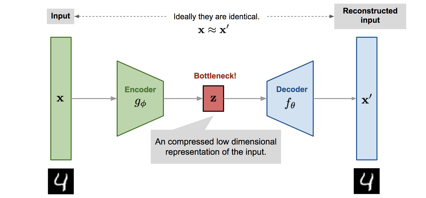
The general Autoencoder architecture consists of two components. An Encoder that compresses the input and a Decoder that tries to reconstruct it.
We'll use the LSTM Autoencoder from this GitHub repo with some small tweaks. Our model's job is to reconstruct Time Series data. Let's start with the Encoder:
class Encoder(nn.Module):

  def __init__(self, seq_len, n_features, embedding_dim=64):
    super(Encoder, self).__init__()

    self.seq_len, self.n_features = seq_len, n_features
    self.embedding_dim, self.hidden_dim = embedding_dim, 2 * embedding_dim

    self.rnn1 = nn.LSTM(
      input_size=n_features,
      hidden_size=self.hidden_dim,
      num_layers=1,
      batch_first=True
    )

    self.rnn2 = nn.LSTM(
      input_size=self.hidden_dim,
      hidden_size=embedding_dim,
      num_layers=1,
      batch_first=True
    )

  def forward(self, x):
    x = x.reshape((1, self.seq_len, self.n_features))

    x, (_, _) = self.rnn1(x)
    x, (hidden_n, _) = self.rnn2(x)

    return hidden_n.reshape((self.n_features, self.embedding_dim))
class Decoder(nn.Module):

  def __init__(self, seq_len, input_dim=64, n_features=1):
    super(Decoder, self).__init__()

    self.seq_len, self.input_dim = seq_len, input_dim
    self.hidden_dim, self.n_features = 2 * input_dim, n_features

    self.rnn1 = nn.LSTM(
      input_size=input_dim,
      hidden_size=input_dim,
      num_layers=1,
      batch_first=True
    )

    self.rnn2 = nn.LSTM(
      input_size=input_dim,
      hidden_size=self.hidden_dim,
      num_layers=1,
      batch_first=True
    )

    self.output_layer = nn.Linear(self.hidden_dim, n_features)

  def forward(self, x):
    x = x.repeat(self.seq_len, self.n_features)
    x = x.reshape((self.n_features, self.seq_len, self.input_dim))

    x, (hidden_n, cell_n) = self.rnn1(x)
    x, (hidden_n, cell_n) = self.rnn2(x)
    x = x.reshape((self.seq_len, self.hidden_dim))

    return self.output_layer(x)
class RecurrentAutoencoder(nn.Module):

  def __init__(self, seq_len, n_features, embedding_dim=64):
    super(RecurrentAutoencoder, self).__init__()

    self.encoder = Encoder(seq_len, n_features, embedding_dim).to(device)
    self.decoder = Decoder(seq_len, embedding_dim, n_features).to(device)

  def forward(self, x):
    x = self.encoder(x)
    x = self.decoder(x)

    return x
model = RecurrentAutoencoder(seq_len, n_features, 128)
model = model.to(device)
def train_model(model, train_dataset, val_dataset, n_epochs):
  optimizer = torch.optim.Adam(model.parameters(), lr=1e-3)
  criterion = nn.L1Loss(reduction='sum').to(device)
  history = dict(train=[], val=[])

  best_model_wts = copy.deepcopy(model.state_dict())
  best_loss = 10000.0

  for epoch in range(1, n_epochs + 1):
    model = model.train()

    train_losses = []
    for seq_true in train_dataset:
      optimizer.zero_grad()

      seq_true = seq_true.to(device)
      seq_pred = model(seq_true)

      loss = criterion(seq_pred, seq_true)

      loss.backward()
      optimizer.step()

      train_losses.append(loss.item())

    val_losses = []
    model = model.eval()
    with torch.no_grad():
      for seq_true in val_dataset:

        seq_true = seq_true.to(device)
        seq_pred = model(seq_true)

        loss = criterion(seq_pred, seq_true)
        val_losses.append(loss.item())

    train_loss = np.mean(train_losses)
    val_loss = np.mean(val_losses)

    history['train'].append(train_loss)
    history['val'].append(val_loss)

    if val_loss < best_loss:
      best_loss = val_loss
      best_model_wts = copy.deepcopy(model.state_dict())

    print(f'Epoch {epoch}: train loss {train_loss} val loss {val_loss}')

  model.load_state_dict(best_model_wts)
  return model.eval(), history
model, history = train_model(
  model,
  train_dataset,
  val_dataset,
  n_epochs=10
)
ax = plt.figure().gca()

ax.plot(history['train'])
ax.plot(history['val'])
plt.ylabel('Loss')
plt.xlabel('Epoch')
plt.legend(['train', 'test'])
plt.title('Loss over training epochs')
plt.show();

MODEL_PATH = 'Time-Series-ECG5000-Pytorch.pth'

torch.save(model, MODEL_PATH)
def predict(model, dataset):
  predictions, losses = [], []
  criterion = nn.L1Loss(reduction='sum').to(device)
  with torch.no_grad():
    model = model.eval()
    for seq_true in dataset:
      seq_true = seq_true.to(device)
      seq_pred = model(seq_true)

      loss = criterion(seq_pred, seq_true)

      predictions.append(seq_pred.cpu().numpy().flatten())
      losses.append(loss.item())
  return predictions, losses
_, losses = predict(model, train_dataset)

sns.distplot(losses, bins=50, kde=True);

THRESHOLD = 26
Normal hearbeats
predictions, pred_losses = predict(model, test_normal_dataset)
sns.distplot(pred_losses, bins=50, kde=True);

correct = sum(l <= THRESHOLD for l in pred_losses)
print(f'Correct normal predictions: {correct}/{len(test_normal_dataset)}')
anomaly_dataset = test_anomaly_dataset[:len(test_normal_dataset)]
predictions, pred_losses = predict(model, anomaly_dataset)
sns.distplot(pred_losses, bins=50, kde=True);

correct = sum(l > THRESHOLD for l in pred_losses)
print(f'Correct anomaly predictions: {correct}/{len(anomaly_dataset)}')
def plot_prediction(data, model, title, ax):
  predictions, pred_losses = predict(model, [data])

  ax.plot(data, label='true')
  ax.plot(predictions[0], label='reconstructed')
  ax.set_title(f'{title} (loss: {np.around(pred_losses[0], 2)})')
  ax.legend()
fig, axs = plt.subplots(
  nrows=2,
  ncols=6,
  sharey=True,
  sharex=True,
  figsize=(24, 8)
)

for i, data in enumerate(test_normal_dataset[:6]):
  plot_prediction(data, model, title='Normal', ax=axs[0, i])

for i, data in enumerate(test_anomaly_dataset[:6]):
  plot_prediction(data, model, title='Anomaly', ax=axs[1, i])

fig.tight_layout();
